Dynamic programming, greedy algorithm and heuristic

A relational database tries the multiple approaches I’ve just said. The real job of an optimizer is to find a good solution on a limited amount of time.

Most of the time an optimizer doesn’t find the best solution but a “good” one.

For small queries, doing a brute force approach is possible. But there is a way to avoid unnecessary computations so that even medium queries can use the brute force approach. This is called dynamic programming.

Dynamic Programming

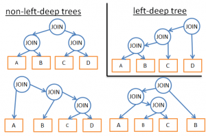
The idea behind these 2 words is that many executions plan are very similar. If you look at the following plans:

They share the same (A JOIN B) subtree. So, instead of computing the cost of this subtree in every plan, we can compute it once, save the computed cost and reuse it when we see this subtree again. More formally, we’re facing an overlapping problem. To avoid the extra-computation of the partial results we’re using memoization.

Using this technique, instead of having a (2*N)!/(N+1)! time complexity, we “just” have 3N. In our previous example with 4 joins, it means passing from 336 ordering to 81. If you take a bigger query with 8 joins (which is not big), it means passing from 57 657 600 to 6561.

For the CS geeks, here is an algorithm I found on the formal course I already gave you. I won’t explain this algorithm so read it only if you already know dynamic programming or if you’re good with algorithms (you’ve been warned!):

For bigger queries you can still do a dynamic programming approach but with extra rules (or heuristics) to remove possibilities:

• If we analyze only a certain type of plan (for example: the left-deep trees) we end up with n*2n instead of 3n

• If we add logical rules to avoid plans for some patterns (like “if a table as an index for the given predicate, don’t try a merge join on the table but only on the index”) it will reduce the number of possibilities without hurting to much the best possible solution.
• If we add rules on the flow (like “perform the join operations BEFORE all the other relational operations”) it also reduces a lot of possibilities.
• …

Greedy algorithms

But for a very big query or to have a very fast answer (but not a very fast query), another type of algorithms is used, the greedy algorithms.

The idea is to follow a rule (or heuristic) to build a query plan in an incremental way. With this rule, a greedy algorithm finds the best solution to a problem one step at a time. The algorithm starts the query plan with one JOIN. Then, at each step, the algorithm adds a new JOIN to the query plan using the same rule.

Let’s take a simple example. Let’s say we have a query with 4 joins on 5 tables (A, B, C, D and E). To simplify the problem we just take the nested join as a possible join. Let’s use the rule “use the join with the lowest cost”

• we arbitrary start on one of the 5 tables (let’s choose A)
• we compute the cost of every join with A (A being the inner or outer relation).
• we find that A JOIN B gives the lowest cost.
• we then compute the cost of every join with the result of A JOIN B (A JOIN B being the inner or outer relation).
• we find that (A JOIN B) JOIN C gives the best cost.
• we then compute the cost of every join with the result of the (A JOIN B) JOIN C …
• ….
• At the end we find the plan (((A JOIN B) JOIN C) JOIN D) JOIN E)

Since we arbitrary started with A, we can apply the same algorithm for B, then C then D then E. We then keep the plan with the lowest cost.

By the way, this algorithm has a name: it’s called the Nearest neighbor algorithm.

I won’t go into details, but with a good modeling and a sort in N*log(N) this problem can easily be solved. The cost of this algorithm is in O(N*log(N)) vs O(3N) for the full dynamic programming version. If you have a big query with 20 joins, it means 26 vs 3 486 784 401, a BIG difference!

The problem with this algorithm is that we assume that finding the best join between 2 tables will give us the best cost if we keep this join and add a new join. But:

• even if A JOIN B gives the best cost between A, B and C
• (A JOIN C) JOIN B might give a better result than (A JOIN B) JOIN C.

To improve the result, you can run multiple greedy algorithms using different rules and keep the best plan.

Other algorithms

[If you’re already fed up with algorithms, skip to the next part, what I’m going to say is not important for the rest of the article]

The problem of finding the best possible plan is an active research topic for many CS researchers. They often try to find better solutions for more precise problems/patterns. For example,

• if the query is a star join (it’s a certain type of multiple-join query), some databases will use a specific algorithm.
• if the query is a parallel query, some databases will use a specific algorithm
• …

Other algorithms are also studied to replace dynamic programming for large queries. Greedy algorithms belong to larger family called heuristic algorithms. A greedy algorithm follows a rule (or heuristic), keeps the solution it found at the previous step and “appends” it to find the solution for the current step. Some algorithms follow a rule and apply it in a step-by-step way but don’t always keep the best solution found in the previous step. They are called heuristic algorithms.

For example, genetic algorithms follow a rule but the best solution of the last step is not often kept:

• A solution represents a possible full query plan
• Instead of one solution (i.e. plan) there are P solutions (i.e. plans) kept at each step.
• 0) P query plans are randomly created
• 1) Only the plans with the best costs are kept
• 2) These best plans are mixed up to produce P news plans
• 3) Some of the P new plans are randomly modified
• 4) The step 1,2,3 are repeated T times
• 5) Then you keep the best plan from the P plans of the last loop.

The more loops you do the better the plan will be.

Is it magic? No, it’s the laws of nature: only the fittest survives!

FYI, genetic algorithms are implemented in PostgreSQL but I wasn’t able to find if they’re used by default.

There are other heuristic algorithms used in databases like Simulated Annealing, Iterative Improvement, Two-Phase Optimization… But I don’t know if they’re currently used in enterprise databases or if they’re only used in research databases.

For more information, you can read the following research article that presents more possible algorithms: Review of Algorithms for the Join Ordering Problem in Database Query Optimization